Most of us have a feeling for what is art and what’s not. But when it comes to its representation we certainly enter a gray area. Does a photograph of a painting has the same value as the original piece? Certainly not. But what about the digital version of an analog photograph? Is it still art or already noise?
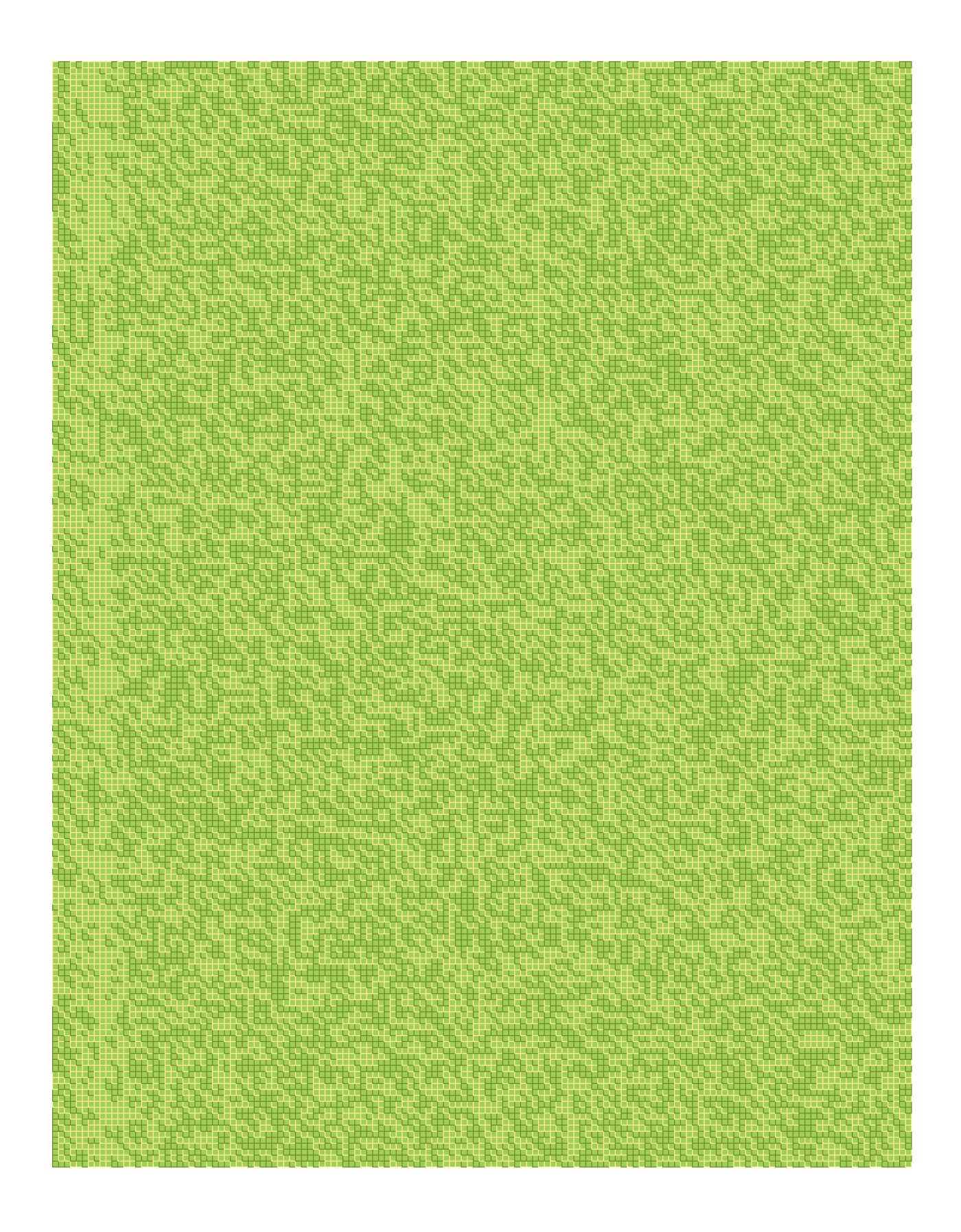
To stress this, I took a JPEG version of Che Guevara’s iconic photograph, turned the ones and zeros of its binary representation into brownish and yellowish lines, and plotted them on an olive-colored background (the same color as his uniform).
The piece I call: the digital revolution.
In this post I will show you how to display the binary representation (also called bit representation) of an arbitrary photograph too.
Introduction
As a prerequisite: I will work on a Debian-based machine (original written using Ubuntu 14 and now tested on my current Devuan Jessie 1.0) and use the languages R and bash.
In addition we need the two bash commands: xxd for making an intermediate hex-dump of the image and the might exiftool to extract its metadata (aspect ratio). Mind that both tools are Linux commands! So the code most probably won’t run on Windows machines or Macs.
While xxd is most probably already available on your system you can install exiftool via
sudo apt install libimage-exiftool-perl
All the following code can be found in a R script in the resources of this blog. It serves as a command line interface and can be called with an image as argument.
# Download the R script
wget https://raw.githubusercontent.com/theGreatWhiteShark/blog-resources/master/art/the-digital-revolution/the-digital-revolution.R

# Download/copy an image in the current folder
wget https://upload.wikimedia.org/wikipedia/commons/thumb/5/58/CheHigh.jpg/113px-CheHigh.jpg

# Execute the R script and supply an image (use one located in the same
# folder or provide the full path instead).
Rscript the-digital-revolution.R 113px-CheHigh.jpg
bash part
To start our project we need an image. As a default one I will use the infamous photograph of Che Guevara. But feel free to choose whatever image and format you like. It does not matter at all.
We’ll use the smallest version available on Wikimedia, since it already contains quite a large number of zeros and ones and we don’t want our output image to be extremely large.
wget https://upload.wikimedia.org/wikipedia/commons/thumb/5/58/CheHigh.jpg/113px-CheHigh.jpg
Now we have to think of a way to access the binary code of the image (every file on the system is actually stored binary). But there is no R function doing this job and it is not as straight forward as I thought it to be. Anyway. What we will do is to convert it into its hexagonal representation. For this we use the Linux program xxd with the option p for a more accessible formatting.
xxd -p 113px-CheHigh.jpg > Che.hex
R part
Now we start a R process. You can do it in the bash by typing R or use some more elaborated platforms like ESS or RStudio (but of course ESS is the better option, since it’s running in Emacs).
First we have to import the hexagonal representation into R and convert it into a binary one. The later task is not an especially hard one, but since we are lazy and want to use a highly optimized code, we let the BMS package handle the job.
che.hex <- read.csv( "./Che.hex", header = FALSE )

install.packages( "BMS" )
require( BMS )

che.bin <- Reduce( c, apply( che.hex, 1, hex2bin ) )
So what just happened? With the read.csv function we imported the hexagonal representation into a data.frame. This is R’s version of a table and the most frequently data type used in this language. Afterwards we used the function apply on the first row of our data.frame che.hex to apply the function hex2bin from the BMS package to each of its elements.
The apply function returns a list holding the binary representations of each single line of the Che.hex file. But this is not really what we want. A single vector containing all the 0 and 1 would be much more appropriate. That’s why we use the Reduce and the c function. With those all elements of the returned list are concatenated to a single vector.
length( che.bin )
Now we have 44008 zeros and ones to work with. Sounds like a nice number.
We could pour these number into any shape but let’s keep the aspect ratio of the original image (113×145).
You can obtain the aspect ratio of your image using the exiftool bash command. Let me stress it: a bash command. So it won’t work in your current R process and you have to open an additional shell to invoke it.
# In the bash
exiftool -ImageSize 113px-CheHigh.jpg
Next, we make a heatmap out of it!
plot.size <- c( NaN, NaN )
plot.size[ 1 ] <- round( sqrt( length( che.bin )* 113/ 145 ) )
plot.size[ 2 ] <- round( plot.size[ 1 ]* 145/ 113 )
che.heatmap.grid <- expand.grid( 1 : plot.size[ 1 ], 1 : plot.size[ 2 ] )
che.heatmap <- data.frame( x = che.heatmap.grid[ , 2 ],
                           y = che.heatmap.grid[ , 1 ],
						   data = che.bin[ 1 : nrow( che.heatmap.grid ) ] )
First we calculate the new pixel numbers along the x and y directions. Then we use the expand.grid function to generate a data.frame containing all the possible permutation of integers between the two sequences. In addition we assign these to a data.frame together with our binary data.
Now we will plot our che.heatmap with the ggplot2 package. If you are using the language R make sure to use this package for plotting. It’s just awesome. Check the links on the official webpage for an introduction.
install.packages( ggplot2 )
require( ggplot2 )
ggplot( data = che.heatmap, aes( x = x, y = y, fill = as.logical( data ) ) ) +
  geom_raster() + scale_fill_manual( values = c( "white", "black" ) )

Okay, now we have our noisy picture. But let’s pimp it up to make it visually more appealing!
ggplot( data = che.heatmap, aes( x = x, y = y, colour = data ) ) + geom_tile()
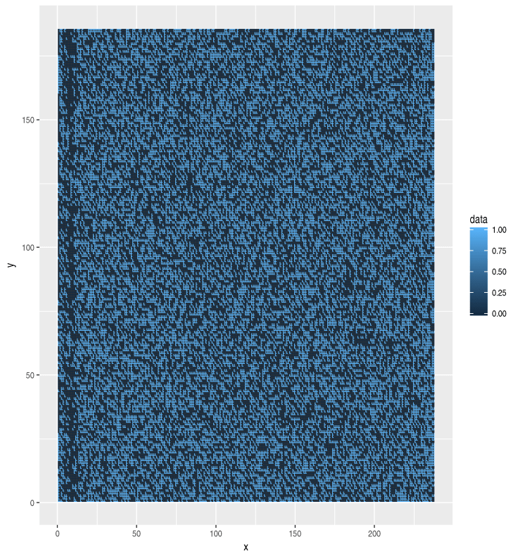
Now this is something we can work with! What happened? We used the two different ways to color a heatmap in ggplot2. The first we filled the individual squares with an uniform color (usually using the fill argument but in this case we used the fallback to the default color) and second we colored the borders separating the squares with two colors (for either 0 or 1) using the colour argument.
ggplot( data = che.heatmap, aes( x = x, y = y, colour = data ) ) +
                geom_tile( fill = "darkolivegreen3") +
    scale_colour_gradientn( colours = c( "khaki1", "olivedrab4" ) ) +
    theme( axis.line = element_blank(),
          axis.text.x = element_blank(),
          axis.text.y = element_blank(),
          axis.ticks = element_blank(),
          axis.title.x = element_blank(),
          axis.title.y = element_blank(),
          legend.position = "none",
          panel.background = element_blank(),
          panel.border = element_blank(),
          panel.grid.major = element_blank(),
          panel.grid.minor = element_blank(),
          plot.background = element_blank() )
ggsave( "che_heatmap.png" , width = 11.3, height = 14.5 )

You can of course choose your own set of colors. 🙂

Leave a comment